SAS-R integration example that I’m giving here is a small and simple one, but I think it represents a model as we proceed into the future of data science. It showcases the fast transformation capabilities of R, and the amazing analytic capabilities of SAS!
SAS-R Integration Example … Because I Was in a Hurry!
Normally, I would not do half a project in R and half a project in SAS! Here is a big picture overview of the problem I was faced with, and how I solved it with this SAS-R integration example:
- I had been developing an analytic dataset from the Behavioral Risk Factor Surveillance Survey (BRFSS) for an analysis of just a subset of records (diabetes patients) – so I didn’t need the population weight variables from BRFSS. I was doing all this in R GUI.
- While we were working on the diabetes paper, the person I was working with got an invitation in her e-mail to submit a paper to a journal on a different topic (healthcare quality) with a very close due date! I realized with just a tweak to my R GUI code, I could redo the current analytic dataset about diabetes that I had been working on, and set up a weighted analysis on the access to care topic!
- I quickly created the access-to-care analytic dataset in R GUI! This accounts for the transformation steps (extract-transform-load, or ETL). But then when I tried to run the weighted analysis in R, it wouldn’t run. It just hung!
- So, I exported a “skinny” dataset out of R GUI into *.csv format. Next, I uploaded it into the free online environment SAS OnDemand for Academics (ODA), which is new!
- I was able to use SAS ODA to convert the *.csv to a SAS dataset, and run PROC SURVEYFREQ on it to get my weighted results!
I’m always trying to show learners a SAS-R integration example that showcases using each tool – SAS and R – optimally for what they are good at. That’s why took the effort of sharing this SAS-R integration example with you. I think it is a perfect illustration of the kind of thinking needed when developing modern SAS data warehouses, as I describe in my book, “Mastering SAS Programming for Data Warehousing”.
SAS-R Integration Example Starts with ETL in R
Transforming data is much simpler in R than SAS, because in SAS, you have to use data step sublanguage which is very complicated. As I recommend in my LinkedIn Learning course in data curation, I first developed a data dictionary for my project that specified the variables in my analytic dataset.
As you can see from the main data dictionary below, the only variables I planned to get from the native dataset were administrative variables having to do with the weighting I needed to do (SEQNO, X_PSU, X_STSTR, X_LLCPWT, and X_STATE), and the access to care variables for the analysis (HLTHPLN1 and MEDCOST).
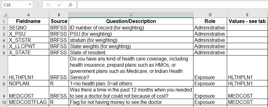
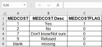
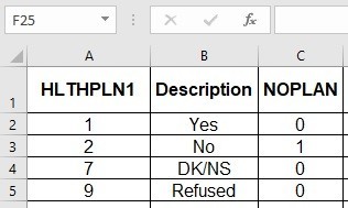
You can also see in the main dictionary that I plan to generate two flag variables in R for analysis: NOPLAN (flag for no health insurance plan), and MEDCOSTFLAG (flag for not having enough money to see a doctor in the last 12 months). Those tabs from the data dictionary are below.
SAS-R Integration Example Data and Code
The original dataset is from the BRFSS 2020 and is in SAS XPT format. You download it from this page, and need to put this huge file in a folder where your computer can access it.
The rest of the data and the code are located on my Github here. The resulting data files are big, so I only included the RDS so you could verify your work.
As you can see with the R GUI code below, the first step is to use the foreign package to convert that bad boy XPT file into an RDS so R can handle it with ease:
# call library(foreign) or load "foreign" package
#that way, we can load the SAS XPT file into R

library(foreign)

#Read XPT directly off of my computer
#and convert it into a dataframe named BRFSS_a.
#You will have to edit this code to add the name of the folder
#where the XPT file is on your computer.

BRFSS_a <- read.xport("C:/NAME OF FOLDER WHERE XPT FILE IS/LLCP2020.xpt")

#check number of columns and rows

colnames(BRFSS_a)
nrow(BRFSS_a)

#export as RDS

saveRDS(BRFSS_a, file = "BRFSS_a.rds")
You will see I import the XPT and export it using naming conventions from my SAS book, which is to advance an alpha suffix: BRFSS_a. Then, in the next code, I read in that BRFSS_a dataset, and start by making a vector called BRFSSVarList with the list of variables from my data dictionary that I know I want to keep:
#read in BRFSS_a

BRFSS_a <- readRDS(file = "BRFSS_a.rds")
colnames(BRFSS_a)

#define varlist
BRFSSVarList <- c("SEQNO", "HLTHPLN1", "MEDCOST", "X_STATE",
"X_PSU", "X_STSTR", "X_LLCPWT")

#subset by varlist
BRFSS_b <- BRFSS_a[BRFSSVarList]

#check columns
colnames(BRFSS_b)

#check rows
nrow(BRFSS_b)

#export as RDS
saveRDS(BRFSS_b, file = "BRFSS_b.rds")
Next, I trim off the variables I don’t need from BRFSS_a by using the BRFSSVarList vector, making the dataframe BRFSS_b – which is now very skinny! I export that as an RDS file.
Referring back to my data dictionary, I realize I need to transform two variables: MEDCOSTFLAG, and NOPLAN, which are both binary flags. I will use that value that equals “1” to designate the numerator of my weighted population percentage in my analysis.
You will see in my transformation code, I read in BRFSS_b, do the transformations (creating the flag variables), advance the transformed dataset to BRFSS_c. Then, to trim off unneeded variables and create analytic datasets in both RDS and CSV format, I first advance to BRFSS_d and then export.
#read in RDS of BRFSS_b

BRFSS_b <- readRDS(file = "BRFSS_b.rds")

#Create flag for no health insurance

BRFSS_b$NOPLAN <- 0
BRFSS_b$NOPLAN [BRFSS_b$HLTHPLN1 !=1 ] <- 1
table(BRFSS_b$NOPLAN, BRFSS_b$HLTHPLN1)

#Create flag for barrier due to cost

BRFSS_b$MEDCOSTFLAG <- 0
BRFSS_b$MEDCOSTFLAG[BRFSS_b$MEDCOST == 1] <- 1
table(BRFSS_b$MEDCOSTFLAG, BRFSS_b$MEDCOST, useNA = c("always")

#advance suffix of data frame
BRFSS_c <- BRFSS_b

#trim off unneeded variables

keep_in_analytic <- c("SEQNO", "X_PSU", "X_STSTR", "X_LLCPWT", "X_STATE",
"NOPLAN", "MEDCOSTFLAG")

BRFSS_d <- BRFSS_c[keep_in_analytic]

#export as an analytic dataset
#in CSV and in RDS

colnames(BRFSS_d)
write.csv(BRFSS_d, file = "access_analytic.csv", row.names = FALSE)
saveRDS(BRFSS_d, file = "access_analytic.rds")

Watch our SAS integration recorded livestreams for use-cases you can apply in your own context!
Doing this strategic renaming of dataframes as we transform creates rollback points in ETL code. The final analytic dataset in CSV format is the one we will put in SAS ODA.
SAS-R Integration Example – Moving on to Analytics in SAS
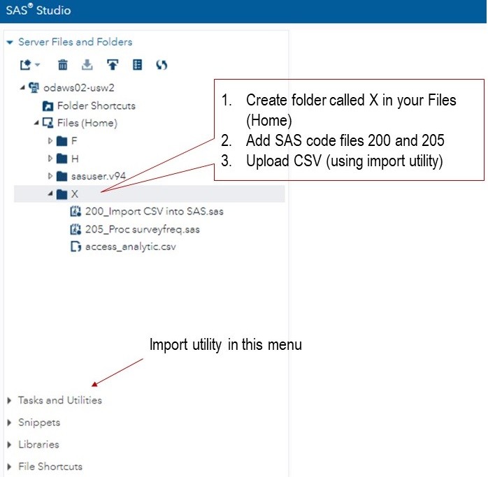
Now we turn to SAS! First, please log into SAS ODA, and upload the files to the right places, as shown in the diagram below. As you can see, you will need to make a folder named X, and we will be mapping a LIBNAME to it. You will need to use the import utility to get the CSV into SAS ODA and converted into a SAS file.
If you are having trouble with this part, please take my free course in using SAS ODA which will help you get set up in SAS ODA. To learn how to get a CSV into SAS, take the second course in the series, “Getting Data into SAS ODA”.
Let’s start by looking at our import code. Because we are transforming data in R and making the analytic dataset into a CSV, we are able to make it light and skinny. However, SAS can’t use the CSV until it converts it with PROC IMPORT. This is a little confusing, in that my course “Getting Data into SAS ODA” teaches you how to get the CSV into the environment, and this code shows you how to convert it to a SAS dataset so SAS can use it.
/*Here, I set LIBNAME to point to folder in SAS ODA*/
/*I made earlier, where I will put data and code for this*/

LIBNAME X "/home/dethwench0/X";
run;

/*Earlier, I used the upload utility to get the CSV into SAS.*/
/*Here, I identify uploaded CSV file as REFFILE to SAS.*/

FILENAME REFFILE '/home/dethwench0/X/access_analytic.csv';

/*PROC IMPORT code: I used the SAS ODA import utility to help me write this code.*/
/*This code converts the REFFILE to a SAS dataset called "analytic"*/
/*and puts it in the X folder mapped to the LIBNAME.*/

PROC IMPORT DATAFILE=REFFILE
DBMS=CSV
OUT=x.analytic;
GETNAMES=YES;
RUN;

/*Here we can review contents of imported SAS dataset*/

PROC CONTENTS DATA=x.analytic;
RUN;
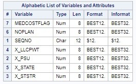
This code outputs the converted SAS dataset to the folder designated by the X LIBNAME, and names it simply analytic. If you are following along, please make sure you edit the example code to point to the folder in your instance of SAS ODA. We also run a PROC CONTENTS to verify that our skinny dataset was uploaded and converted to SAS format successfully. Here is some of our PROC CONTENTS output:
Also, after you edit and run that code successfully, you will notice that the converted SAS file analytic.sas7bdat will show up in your X folder.
Leveraging SAS’s Analytics Capabilities in SAS-R Integration Example
Now we get to the part where we showcase SAS’s analytics abilities. As I said before, the CDC offers guidance on how to do a weighted analysis of BRFSS data in both R and SAS. When I originally tried this in R GUI, I used the code provided by the CDC, and it just was not efficient enough on my system to run. It hung!
That’s the problem with R – it can’t handle big data analytics like SAS can. In fact, I was lucky to be able to do this SAS-R integration example, because the source BRFSS dataset was big, but not too big. If it had been too big to get into R GUI, I would definitely have not been able to put it in SAS ODA. I would have probably needed a SQL server instance at that point!
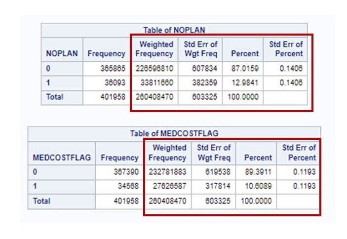
But now that we could provide SAS a manicured analytic dataset, it handled our weighted frequency analysis with ease in PROC SURVEYFREQ:
/*just to make sure LIBNAME is mapped*/
LIBNAME X "/home/dethwench0/X";
run;

/*Running PROC SURVEYFREQ on access to care variables*/
/*in "skinny" analytic dataset prepared in R and uploaded as CSV*/
/*Code provided by BRFSS/CDC for modification. That way, I knew*
/*I put the stratum variables in the right options.*/

proc surveyfreq
	data = x.analytic;
/* Use common weight because both questions are from the core section */
	weight x_llcpwt;
	strata x_ststr;
	cluster x_psu;
table noplan;
table medcostflag;
run;
I ran this code and got the output I needed from PROC SURVEYFREQ – which was the weighted estimates. I show you below:
Remember, if you are getting started with either R or SAS, or just data science in general, take my courses on LinkedIn Learning. They are great for beginners new to data science who have experience in other fields.
Updated December 26, 2021. Added videos, updated links, and added banners on March 4, 2024.
Read all of our data science blog posts!
Looking for a SAS-R integration example that uses the best of both worlds? I show you a use-case where I was in a hurry, and did transformation in R with the analysis in SAS!
